Dr. Brad Muller
The WSR-88D measures
radial velocities in addition to reflectivity by measuring
the Doppler effect
on the radar beam. The Doppler effect is that when a
target (usually precipitation in the case of a weather
radar) is moving away from the radar, the wavelength of the
return echo is longer than
that of the emitted electromagnetic pulse. When the
target is moving toward the radar, the return echo has a shorter wavelength than that of the
emitted pulse (seen in this slide from NWS Milwaukee):
In theory, the wavelength (or frequency) shift can be used to calculate a doppler velocity (see Doppler Radar Formulas) which is the component of movement either toward or away from the radar, also called the radial velocity.
According to Doppler radar theory (see Federal Meteorological Handbook 11, Part-B, pages A-6 to A-8), the wavelength or frequency shift is related to a phase shift in the signal.
In practice, the phase shift between the outgoing and its return signal caused by movement of targets (i.e., precipitation) is too small (on the order of 0.01 degrees for a velocity of 1 m/s) to measure accurately for typical meteorological velocities. Because of this, the NEXRAD measures the phase shift from pulse to pulse caused by differences in positions of the targets over the period between the pulses, which is a much larger angle (on the order of 1 degree). Calculation of the phase shift between two pulses allows calculation of the difference in the range, r (distance from the radar along the beam) to the target between the two pulses. Since velocity is just change of position per unit time (in this case Vr = dr/dt) the change in phase between the two pulses gives us the radial velocity.
Radial velocity is the component of wind velocity parallel to the direction of the radar beam either toward or away from the radar.
Radial velocities are defined as (+) when they are moving away from the radar (outbound).
Radial velocities are defined as (-) when they are moving toward the radar (inbound).
The figure below shows the relationship of wind and radial velocity:
Vr = V cos (theta) =
V cos (0) = V x 1 = V
In this case the radar sees "all" of the wind--the radial velocity is the actual velocity.
Perpendicular (wind at right angles to the beam)
Vr = V cos (theta) = V cos (90) = V x 0 = 0
In this case the radar cannot "see" any of the wind (radial velocity is zero) because there is no component along the beam.
A typical relatively uniform wind field shows radial velocities at a maximum when the radar beam is lined up with the wind direction, and zero when it is perpendicular (as seen in the following slide from the NWS Milwaukee NEXRAD tutorial):
Note that the general wind direction can be discerned as perpendicular to the "zero isodop," and on a line between the incoming and outgoing wind maxima.
This link shows a variety of idealized wind patterns and how they would be appear in terms of radial velocity on a PPI (from the National Severe Storms Laboratory A Guide for Interpreting Doppler Velocity Patterns Northern Hemisphere Edition). There are two main considerations in the radial velocity patterns that emerge:
(1) how the beam is oriented in relation to the wind direction at any given location
(2) vertical shear of the wind speed or direction, since the elevation of the radar beam above ground level increases with distance from the radar
Idealized examples from
https://www.nssl.noaa.gov/publications/dopplerguide/chapter2.php
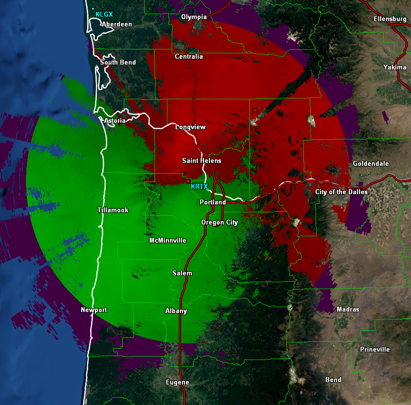
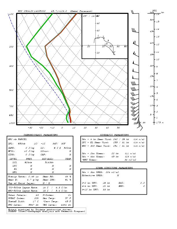
The following example of radial velocity from the Portland, Oregon NEXRAD site and an accompanying model wind sounding illustrates how some of the idealized concepts apply in a real weather situation. Note the shift of the orientation of the zero isodop with range in conjunction with vertical wind shear in the sounding. Low-level winds are southerly, but shift to southwesterly aloft.
Velocity examples (N0U) from Hurricane Michael Landfall:
Michael landfall radial velocity animation.
Michael landfall reflectivity animation.
Simple Applications of Doppler Velocity:
Improved detection of severe weather was the primary budgetary justification for NEXRAD; this includes the detection of microburst divergence and tornadic rotation.
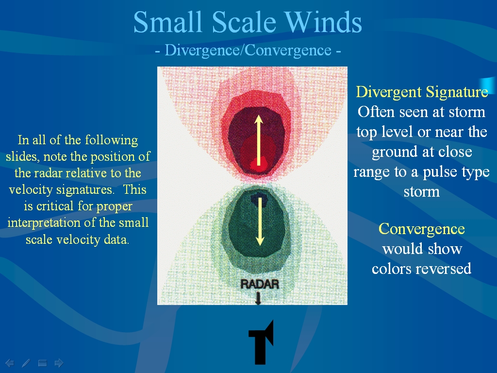
Divergence
Divergence associated with microbursts and downbursts can be detected as signatures of outbound doppler velocities in close proximity to inbound signatures along the line of the radar beam. The inbound winds are closer to the radar, with outbound winds slightly farther (the reverse, with inbound farther and outbound closer would be a convergent signature).
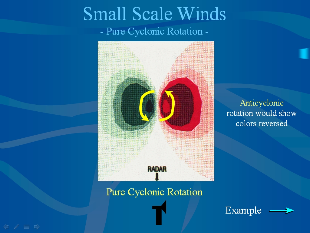
Rotation:
Rotational signatures are seen as side-by-side outbound and inbound doppler velocities in close proximity across the radar beam:
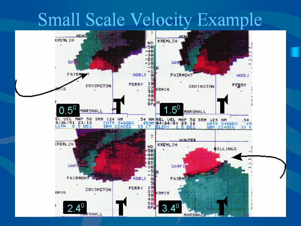
Example: Rotation at the bottom of the storm, divergence at the top:
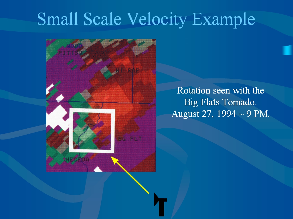
Tornadic rotational velocities:
Storm-Relative vs. Base Velocity:
Base velocity is just the ground-relative radial velocity that is directly measured by the doppler radar. Microburst and downburst signatures of straightline winds are best seen using the base velocity. In GARP, base velocity for the 0.5 degree tilt is N0V.
Storm-relative velocity has the storm motion subtracted out of the base velocity, leaving the storm- relative motion:
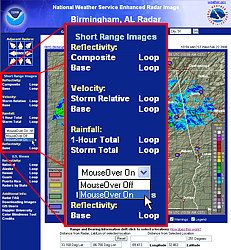
The NWS radar displays on the Internet present both Base Velocity and Storm Relative Velocity:
In theory, the wavelength (or frequency) shift can be used to calculate a doppler velocity (see Doppler Radar Formulas) which is the component of movement either toward or away from the radar, also called the radial velocity.
According to Doppler radar theory (see Federal Meteorological Handbook 11, Part-B, pages A-6 to A-8), the wavelength or frequency shift is related to a phase shift in the signal.
In practice, the phase shift between the outgoing and its return signal caused by movement of targets (i.e., precipitation) is too small (on the order of 0.01 degrees for a velocity of 1 m/s) to measure accurately for typical meteorological velocities. Because of this, the NEXRAD measures the phase shift from pulse to pulse caused by differences in positions of the targets over the period between the pulses, which is a much larger angle (on the order of 1 degree). Calculation of the phase shift between two pulses allows calculation of the difference in the range, r (distance from the radar along the beam) to the target between the two pulses. Since velocity is just change of position per unit time (in this case Vr = dr/dt) the change in phase between the two pulses gives us the radial velocity.
Radial velocity is the component of wind velocity parallel to the direction of the radar beam either toward or away from the radar.
Radial velocities are defined as (+) when they are moving away from the radar (outbound).
Radial velocities are defined as (-) when they are moving toward the radar (inbound).
The figure below shows the relationship of wind and radial velocity:
The magnitude of the
wind components toward or away from the radar along the
radial, i.e., the radial velocity (Vr)
are given by
Vr = V
cos (theta)
where V is the actual wind speed, and theta is the angle between the wind direction and the radial.
We can analyze this relationship by examine the two simple cases of winds exactly parallel to the radar beam and winds perpendicular to it.
Parallel (wind exactly along the beam)
where V is the actual wind speed, and theta is the angle between the wind direction and the radial.
We can analyze this relationship by examine the two simple cases of winds exactly parallel to the radar beam and winds perpendicular to it.
Parallel (wind exactly along the beam)
In this case the radar sees "all" of the wind--the radial velocity is the actual velocity.
Perpendicular (wind at right angles to the beam)
Vr = V cos (theta) = V cos (90) = V x 0 = 0
In this case the radar cannot "see" any of the wind (radial velocity is zero) because there is no component along the beam.
A typical relatively uniform wind field shows radial velocities at a maximum when the radar beam is lined up with the wind direction, and zero when it is perpendicular (as seen in the following slide from the NWS Milwaukee NEXRAD tutorial):
Note that the general wind direction can be discerned as perpendicular to the "zero isodop," and on a line between the incoming and outgoing wind maxima.
This link shows a variety of idealized wind patterns and how they would be appear in terms of radial velocity on a PPI (from the National Severe Storms Laboratory A Guide for Interpreting Doppler Velocity Patterns Northern Hemisphere Edition). There are two main considerations in the radial velocity patterns that emerge:
(1) how the beam is oriented in relation to the wind direction at any given location
(2) vertical shear of the wind speed or direction, since the elevation of the radar beam above ground level increases with distance from the radar
Idealized examples from
https://www.nssl.noaa.gov/publications/dopplerguide/chapter2.php
The following example of radial velocity from the Portland, Oregon NEXRAD site and an accompanying model wind sounding illustrates how some of the idealized concepts apply in a real weather situation. Note the shift of the orientation of the zero isodop with range in conjunction with vertical wind shear in the sounding. Low-level winds are southerly, but shift to southwesterly aloft.
Velocity examples (N0U) from Hurricane Michael Landfall:
Michael landfall radial velocity animation.
Michael landfall reflectivity animation.
Simple Applications of Doppler Velocity:
Improved detection of severe weather was the primary budgetary justification for NEXRAD; this includes the detection of microburst divergence and tornadic rotation.
Divergence
Divergence associated with microbursts and downbursts can be detected as signatures of outbound doppler velocities in close proximity to inbound signatures along the line of the radar beam. The inbound winds are closer to the radar, with outbound winds slightly farther (the reverse, with inbound farther and outbound closer would be a convergent signature).
Rotation:
Rotational signatures are seen as side-by-side outbound and inbound doppler velocities in close proximity across the radar beam:
Example: Rotation at the bottom of the storm, divergence at the top:
Tornadic rotational velocities:
Storm-Relative vs. Base Velocity:
Base velocity is just the ground-relative radial velocity that is directly measured by the doppler radar. Microburst and downburst signatures of straightline winds are best seen using the base velocity. In GARP, base velocity for the 0.5 degree tilt is N0V.
Storm-relative velocity has the storm motion subtracted out of the base velocity, leaving the storm- relative motion:
base velocity =
storm-relative velocity + storm motion
or
storm-relative velocity = base velocity - storm motion
Rotational signatures such as tornadoes
and
supercells
(if necessary hit shift-reload to animate)
are best seen using the storm-relative velocity
(from an NWS Melbourne storm
survey of the Feb. 2007 central Florida Groundhog Day
tornado). In GARP, storm-relative velocity
for the .5 degree tilt is N0S.or
storm-relative velocity = base velocity - storm motion
This can be
visualized by imagining you are riding along with a
supercell thunderstorm (mesocyclone). The
storm-relative motion is the circulating motion you
would see in the storm around you, i.e., the rotation.
In the following example from the Oklahoma Climatological Survey, the base velocity is the "Resultant Flow Pattern" and subtracting out the storm motion yields the storm-relative velocity which is depicted as the "Mesocyclonic Circulation." It is these kind of circulations one is looking for in trying to detect potentially tornadic thunderstorms.
In the following example from the Oklahoma Climatological Survey, the base velocity is the "Resultant Flow Pattern" and subtracting out the storm motion yields the storm-relative velocity which is depicted as the "Mesocyclonic Circulation." It is these kind of circulations one is looking for in trying to detect potentially tornadic thunderstorms.
The NWS radar displays on the Internet present both Base Velocity and Storm Relative Velocity:
The following
examples show how storm-relative velocity enhances
our ability to recognize the rotation of a supercell
storm over the base velocity.
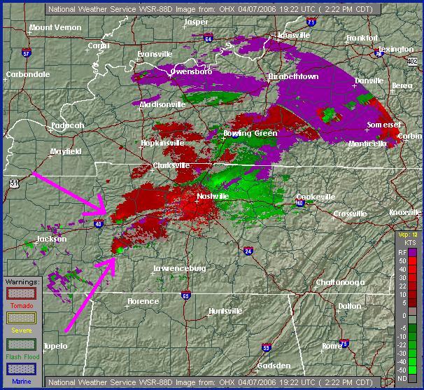
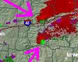
Base velocity image of a pair of supercell thunderstorms. The storms are moving rapidly from southwest to northeast toward the Nashville radar so the base velocity images indicate all inbound velocities in these supercells:
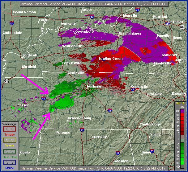
Storm-relative velocity shows rotating supercells much more clearly because the ground-motion of the storm has been subtracted out. Relative to movement with the storm, the rotation can be seen in the side-by-side doppler velocity couplets of outbound and inbound winds in close proximity
Base velocity image of a pair of supercell thunderstorms. The storms are moving rapidly from southwest to northeast toward the Nashville radar so the base velocity images indicate all inbound velocities in these supercells:
Storm-relative velocity shows rotating supercells much more clearly because the ground-motion of the storm has been subtracted out. Relative to movement with the storm, the rotation can be seen in the side-by-side doppler velocity couplets of outbound and inbound winds in close proximity
Many examples of
rotational signatures of storm-relative velocity from
the 1998
Central Florida Tornado Outbreak can be found here.
This was the deadliest
tornado outbreak in Florida history, killing 42
people.