Remote Sensing--Making measurements from a distance. Passive remote sensing makes measurements of naturally-occurring radiation at a distance from the objects being observed. Active remote sensing sends out pulses of electromagnetic radiation and measures radiation that bounces back to the sensor from the object.
Weather satellites generally make passive radiation measurements at a distance from the earth and atmosphere.
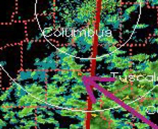
Weather radars make active radiation measurements of precipitation suspended in the air.
Remote sensing from satellites and weather radars provides several advantages over conventional (surface and radiosonde) observations:
(1) Data over oceans and other areas not well covered by conventional obs.
(2) Data between conventional observation stations, even in well covered areas.
(3) More frequent
observations.
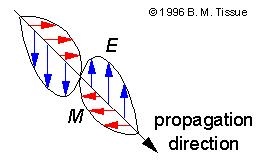
Radiation--Transfer of energy through space by electromagnetic waves.
Electromagnetic waves are up and down fluctuations in the energy levels of electromagnetic fields.
Basics of Electromagnetic Radiation
1. All substances with a temperature above absolute zero emit electromagnetic (EM) radiation (with the exception of so-called dark matter which has been theorized to provide the unobserved mass needed to account for observed motions of astrophysical bodies such as galaxies).
2. EM radiation travels at the speed of light (co
= 2.99792458 x 10⁸ m s-1 in a vacuum,
slightly slower in air) and is characterized by its
(1) wavelength (![]() )--distance from wavecrest to wavecrest.
)--distance from wavecrest to wavecrest.
(2) frequency ( ![]() )--no.
wavecrests passing a certain point over a given period of time.
Wavelength is related to frequency by
)--no.
wavecrests passing a certain point over a given period of time.
Wavelength is related to frequency by

Note: Wavelength is inversely proportional to frequency--longer wavelength radiation has lower frequency; shorter wavelength radiation has higher frequency.
(3) amplitude--magnitude of
the wave, i.e., maximum displacement from the "zero" energy
level to the peak energy level; it is a measure of the intensity
(i.e. the strength) of the electromagnetic radiation.
To see interactive animations illustrating wavelength, frequency, and amplitude, click on the following links:
Basic
Electromagnetic Wave Properties--Olympus America's Microscopy
Resource Center.
Electromagnetic Radiation--Olympus America's Microscopy Resource Center.
[(4) An additional related way of describing EM radiation is wavenumber which is the number of wavecrests per unit distance, usually given in cm-1.]
3. EM Spectrum--all the different wavelengths
from very short to very long.
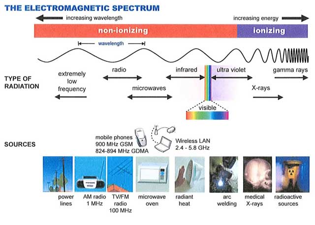
(1) The shorter the wavelength of the radiation, the higher is its energy level "per wave". Thus X-Rays carry much more energy than microwaves, for example.
(2) Visible light is the portion of the spectrum of wavelengths from 0.4-0.7 micrometers.
(3) Ultraviolet (UV) radiation is at wavelengths from 0.1 -0.4 micrometers.
(4) Near Infrared (IR) is 0.7-4.0 micrometers.
(5) IR is roughly 4.0-1000 micrometers.
(6) For weather satellites we we will be mainly concerned with the visible and IR portions of the spectrum up to about 20 micrometers. For weather radar we will be concerned with the microwave part of the spectrum at wavelengths 3-10 cm.
5. Radiation Concepts and Definitions:
(1) Emission --
Radiant energy emanating from an object. At a given wavelength,
we represent emission by ![]() , where the lambda subscript denotes a
single wavelength.
, where the lambda subscript denotes a
single wavelength.
(2) Absorption (![]() )--Removal of radiant energy from
a beam incident on an object and conversion into internal energy
(heat) of the absorbing object, where
)--Removal of radiant energy from
a beam incident on an object and conversion into internal energy
(heat) of the absorbing object, where
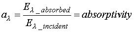
is the fractional amount of the incident radiation that is absorbed.
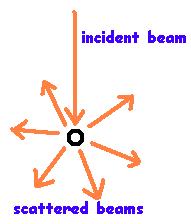
(3) Scattering--Continuous removal of energy from a beam of radiation incident on an object and reradiation of that energy in all directions.
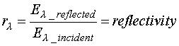
(4) Transmission (![]() )--That portion of a radiation
beam that is neither absorbed nor scattered and continues
unimpeded through a translucent medium, where
)--That portion of a radiation
beam that is neither absorbed nor scattered and continues
unimpeded through a translucent medium, where
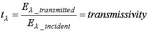
In considering a beam of radiation incident upon a translucent medium such as the atmosphere, all the radiation has to be accounted for, so that all fractional amounts add up to 1:
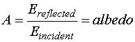
(5) Albedo (A)--The ratio of the amount of electromagnetic radiation reflected by an object in comparison with the amount striking it. Usually, the term is used in conjunction with the visible light part of the spectrum, so it refers to the fraction of visible light reflected by an object relative to the amount incident on the object. It can also be expressed as a percentage.
(1) Planck's Law:
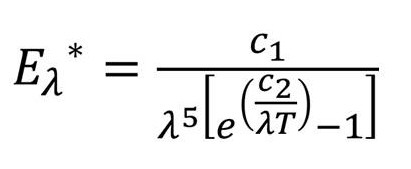
where T is absolute temperature in Kelvin (K) and the asterisk indicates blackbody emission,
c1= 3.74 x 10⁸ W m-2 micrometers4
c2=1.44 x 10⁴ micrometers K
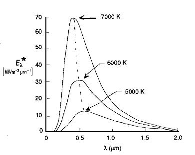
The Planck Function gives radiative flux as a function of wavelength and temperature for "blackbody" radiation. It shows how much radiation at a particular wavelength per unit surface area would be emitted by an object based on its temperature, assuming it is emitting the maximum possible radiation, i.e., it is a "perfect" emitter. Actual objects are not perfect emitters, so actual emission at a given wavelength typically is less than the blackbody value:
The figure below shows the Planck function
plotted for three different temperatures:
(2) Stefan-Boltzmann Law: Obtained by integrating the Planck Function with respect to wavelength across the entire spectrum.
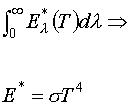
where ![]() is the Stefan-Boltzmann constant = 5.67 x 10⁻⁸
W m-2 K-4 and E* has units of W m-2.
It is the area under the curve of the Planck Function.
It says that the total radiant energy emitted by an object
across all wavelegths is proportional to the fourth
power of temperature of the object. The warmer the object, the
greater is its radiant energy output.
is the Stefan-Boltzmann constant = 5.67 x 10⁻⁸
W m-2 K-4 and E* has units of W m-2.
It is the area under the curve of the Planck Function.
It says that the total radiant energy emitted by an object
across all wavelegths is proportional to the fourth
power of temperature of the object. The warmer the object, the
greater is its radiant energy output.
(3) Wien's Law: Obtained by differentiating the Planck Function with respect to wavelength, and setting it equal to zero. The wavelength of maximum emission is found where the slope of the Planck Function curve is equal to zero:
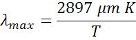
Wien's Law says that the wavelength of maximum emission by an object is inversely proportional to the temperature of the object. The warmer the object, the shorter will be its wavelength of maximum emission.
(3) Kirchoff's Law: For an object in local thermodynamic equilibrium, radiation absorptivity equals radiation emissivity at a particular wavelength.
![]()
It says that efficient
absorbers are efficient emitters at a particular wavelength and
poor absorbers are poor emitters at a particular wavelength.
Example: Radiation in
the wavelength band around 6.7 micrometers (part of the IR
spectrum) is strongly absorbed by water vapor. This means
that water vapor also strongly emits radiation in this part of
the spectrum. This fact is exploited by the 6.7 micrometer
water vapor channels on weather satellites--they measure
radiation that has been emitted by middle and upper tropospheric
water vapor.
7. Transmission of Radiation in the Earth's Atmosphere
(1) The earth's atmosphere does not behave like a blackbody, absorbing and emitting with nearly 100% efficiency. Instead it contains some wavelength bands in which it absorbs nearly all the radiation, and others in which it transmits nearly all the radiation; the numbered boxes on the image below refer roughly to the spectral regions measured by the heritage GOES-Imager radiometers carried on GOES satellites up through GOES-15.
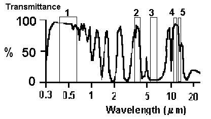
(2) Any specific portion of the EM spectrum is called a spectral band; those in which radiation is strongly absorbed by the atmosphere are called absorption bands.
(3) Different constituents of the atmosphere have different absorption/emission properties and thus are responsible for different (sometimes overlapping) absorption bands. All are superimposed together to determine the total atmospheric absorption and transmission of radiation.
(4) Spectral bands in which little absorption takes place are called window regions, because most of the radiation is transmitted rather than absorbed.
(5) For the infrared portion of the spectrum, the most important absorption bands are due to carbon dioxide (CO2) and water vapor (H2O).
(6) The different weather satellite radiometer channels are chosen to exploit the reflection characteristics of the surface and clouds, or the emission characteristics of ocean, land, and cloud surfaces, in combination with the transmission characteristics of the atmosphere. The numbers 1-5 in the atmospheric spectrum depicted above show the spectral positions of the GOES imager channels.
8. Weather Satellite Channels.
There are four broad
categories of imaging weather satellite channels; they are
listed below, along with the physical process that are the
source of the radiation measured by channels in that category:
1) visible;
reflection of solar radiation
2) near-IR/shortwave IR;
both reflection of "shortwave" solar radiation and thermal
emission of "shortwave" radiation; this NASA video
provides a good summary of this part of the spectrum
3) water vapor; emission
of radiation in the the water vapor absorption band of the
thermal IR part of the spectrum, and
4) IR; thermal emission of
"longwave" IR radiation
Visible, water vapor, and IR
are the ones most commonly used in weather analysis and
forecasting. The "heritage"
GOES-Imager on the GOES-I-P series
(GOES-8 through GOES-15) contained one visible channel, one
near-IR channel, one water vapor channel, one "clean" IR window
channel, and a "dirty" IR window channel (while it was a window
channel, there is also significant absorption by water vapor in
this band of the spectrum), and then later an IR window "CO2
channel," that, while a window, also experiences significant
absorption by CO2.
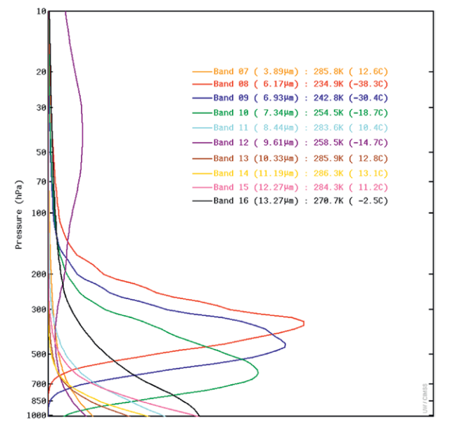
Starting with GOES-16,
and now GOES-17, the GOES satellites carry the Advanced Baseline
Imager (ABI), a 16-channel radiometer with heritage of
wavelengths both from previous GOES generations, and also
polar-orbiting satellites such as the AVHRR (Advanced Very High
Resolution Radiometer), and MODIS (MODerate resolution Imaging
Spectroradiometer)
The following is a brief overview of the "heritage" visible, IR, and water vapor channels, and their analogs on the ABI, which are shown in bold:
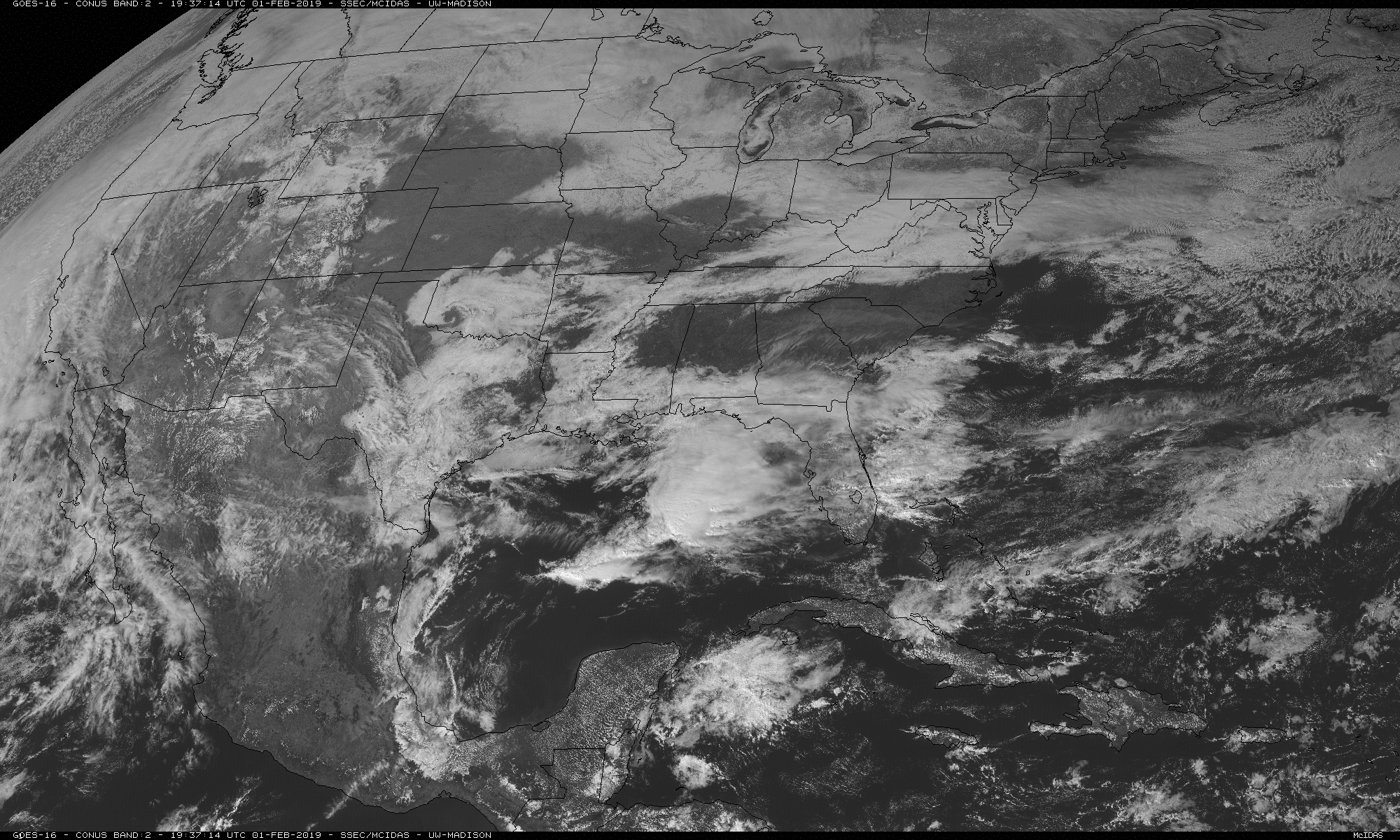
(1) Visible channels (heritage GOES Imager Channel 1, centered at 0.65 micrometers [red], ABI Channel 2 0.64 micrometers [red], and ABI Channel 1 0.47 micrometers [blue].
A. Sensitive to radiation in the visible part of the spectrum.
B. They depend on reflection of sunlight by the earth's surface and clouds.
- Higher albedo surfaces appear light in black and white visible imagery
- Lower albedo surfaces appear dark in black and white visible imagery.
C. Both low and high clouds appear bright.
D. Cannot be used at night.
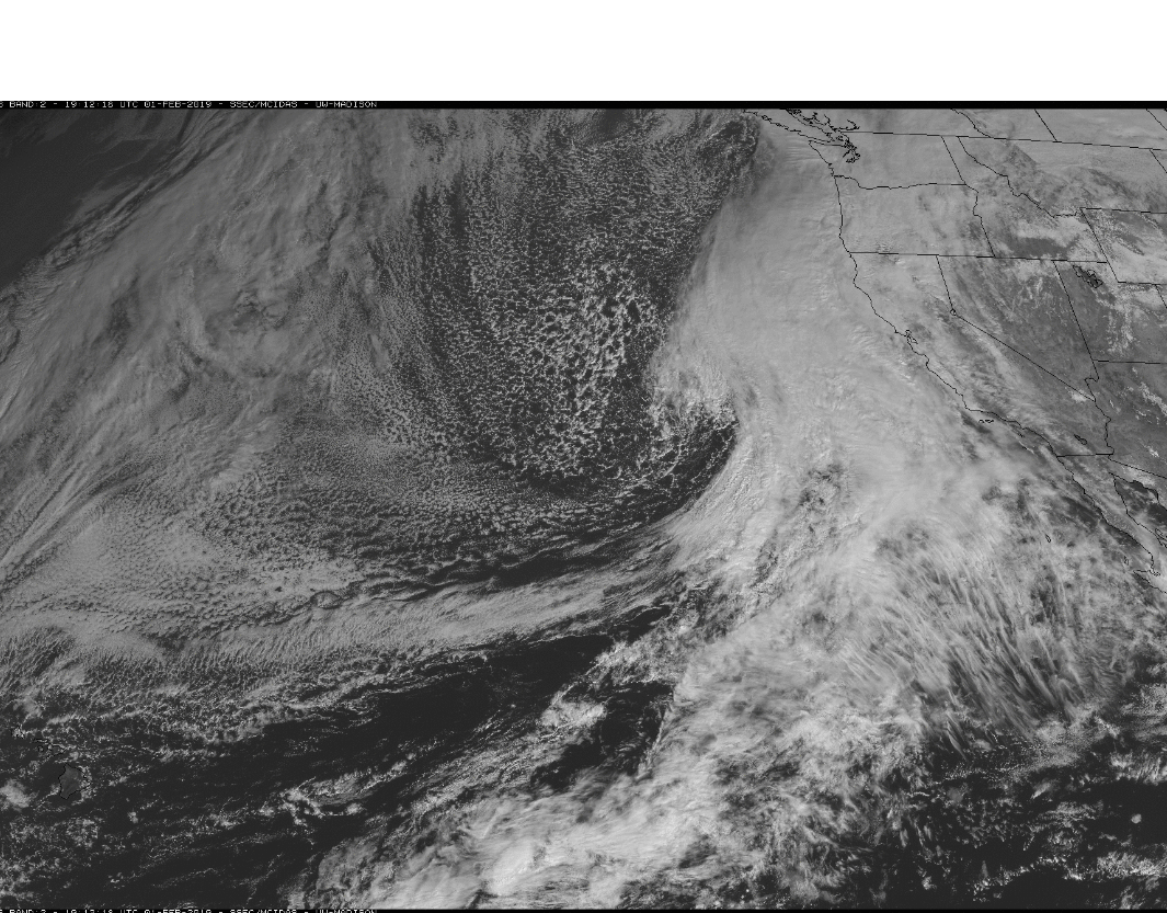
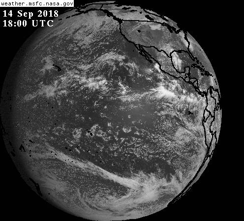
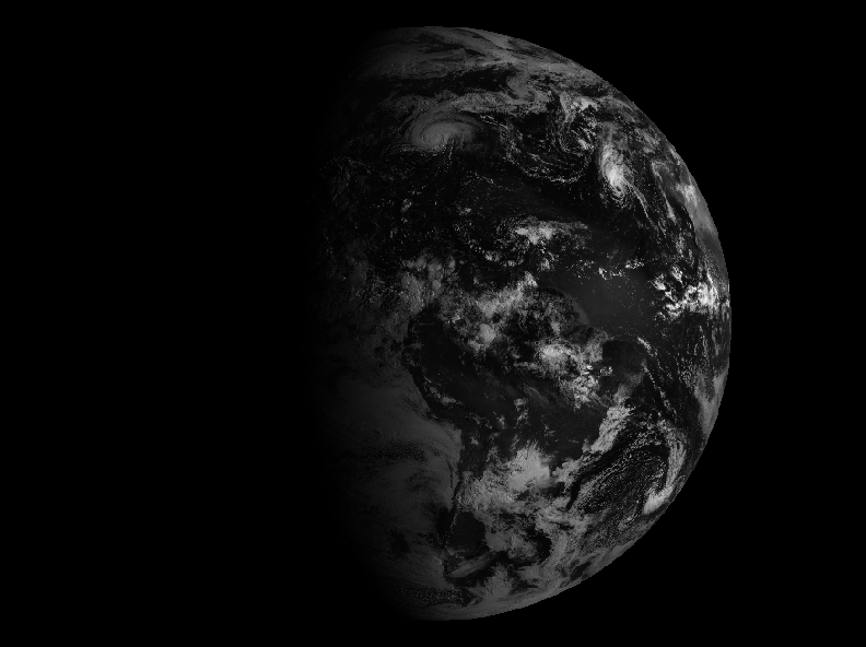
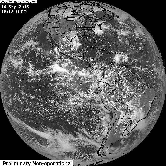
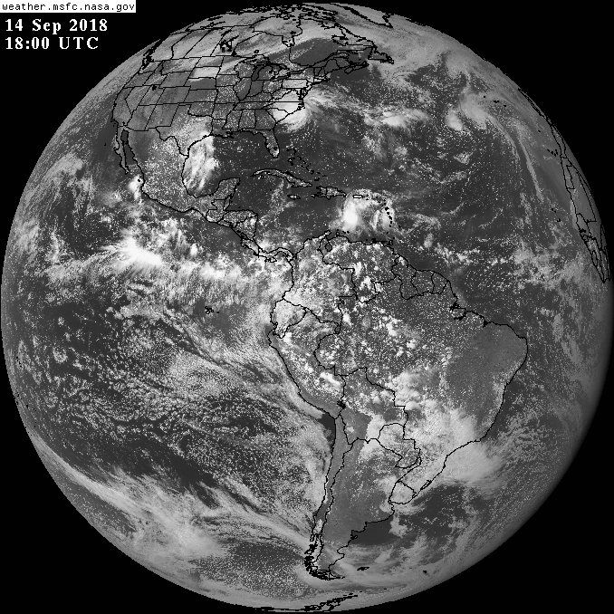
Example of a heritage visible 0.65 micrometer image from GOES-11. Ocean has low albedo and appears dark; clouds have high albedo and appear bright. The day/night line or terminator is evident from northwestern Canada to just west of Hawaii.
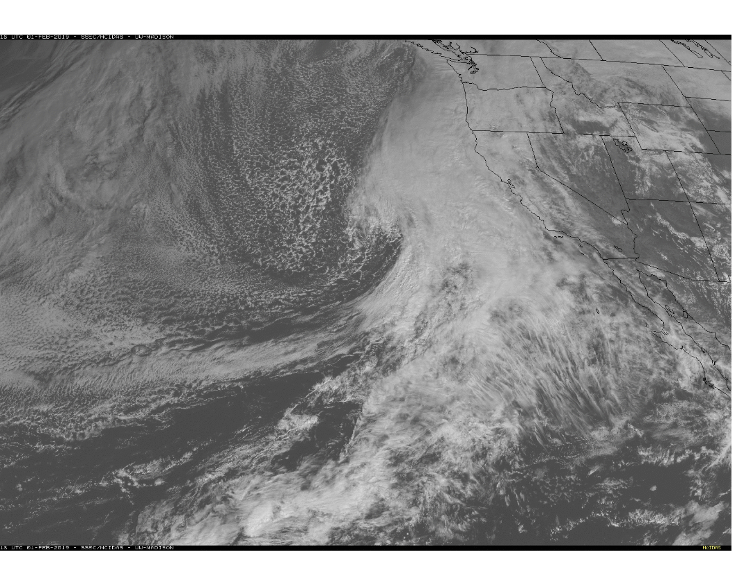
Example of a red 0.64 micrometer ABI Channel 2 VIS from the GOES-17:
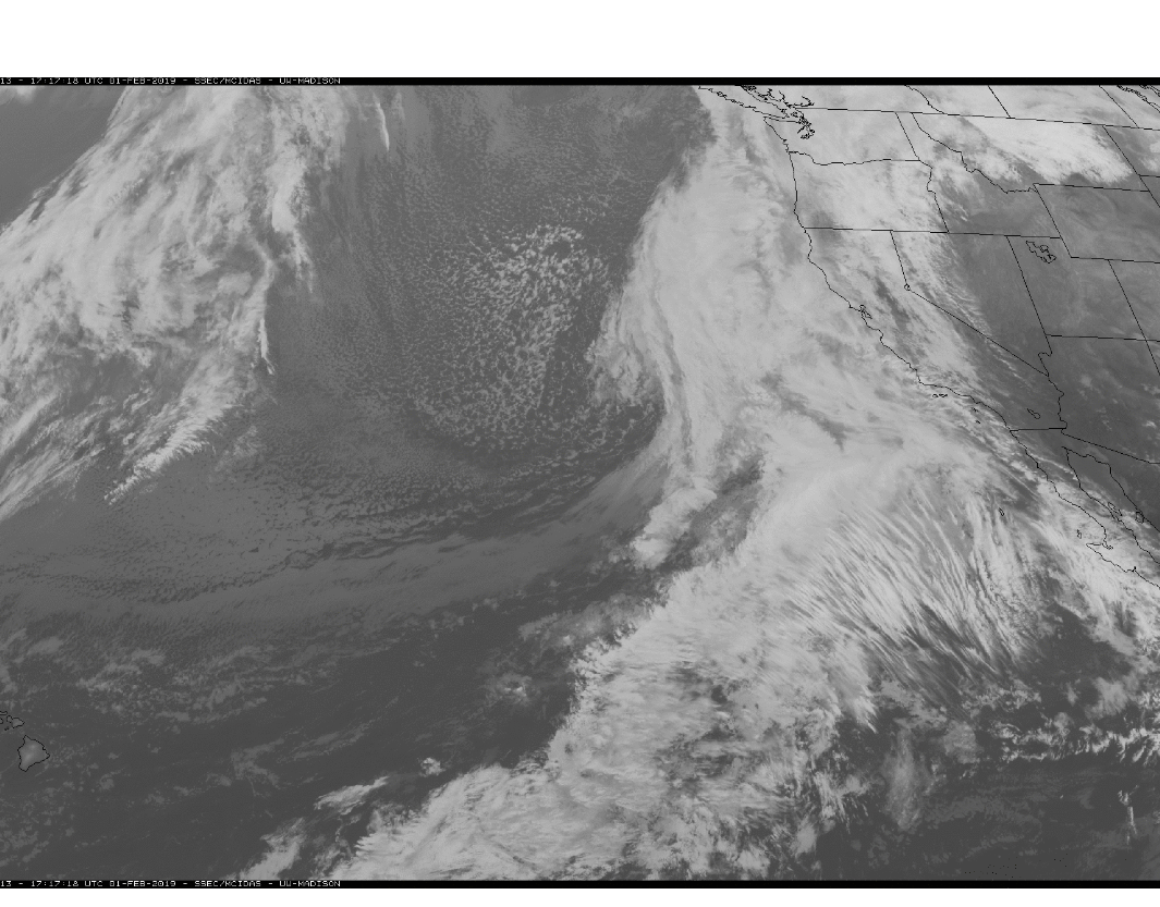
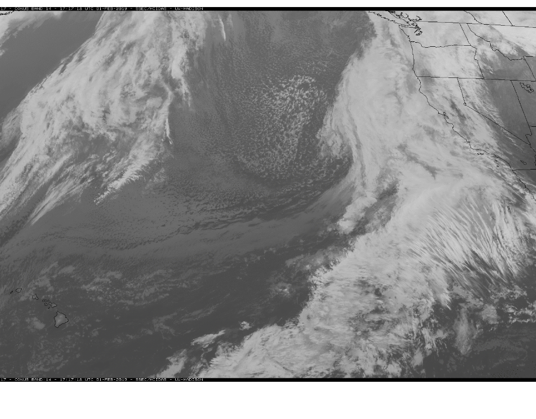
(2) Conventional infrared (IR) channels (heritage GOES Imager Channel 4, centered at 10.7 micrometers, ABI Channel 13 10.3 micrometer clean longwave window, ABI Channel 14 11.2 micrometer IR longwave window,).
Example of a blue 0.47 micrometer ABI Channel 1 VIS from the GOES-17:
Note that the greyer, hazier, more "washed out" look of the blue channel is due to more atmospheric scattering of the shorter blue wavelengths, than of the red wavelengths of the previous image.
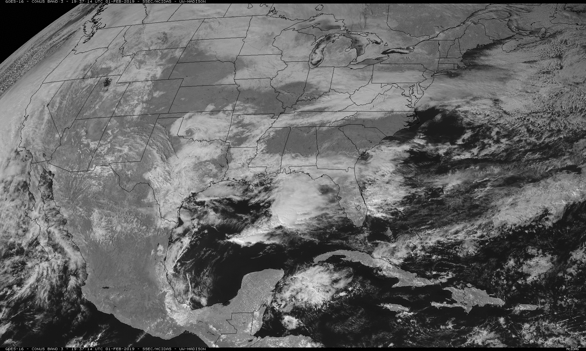
To make a full color visible image similar to what our eyes would see from the satellite vantage point, one must have input from the three primary colors of light, red, blue, and green wavelengths. Since there is no green channel on the ABI, we use a near IR ABI channel 3 at 0.86 micrometers with significant reflection from vegetation (the so-called "veggie" channel) as a surrogate (i.e., a substitute) for green. There is actually considerably more reflection from vegetation at 0.86 micrometers than there is at green wavelengths, so the 0.86 micrometer input to green must be "toned down" to balance with the input from the blue and red ABI channels to make realistic-looking visible color imagery:
GOES-16 ABI Channel 1 (blue):
GOES-16 ABI Channel 2 (red):
GOES-16 Channel 3 near IR 0.86 micrometer (surrogate for green); note the brightness of the land surfaces due to the high reflectivity of vegetation at this wavelength:
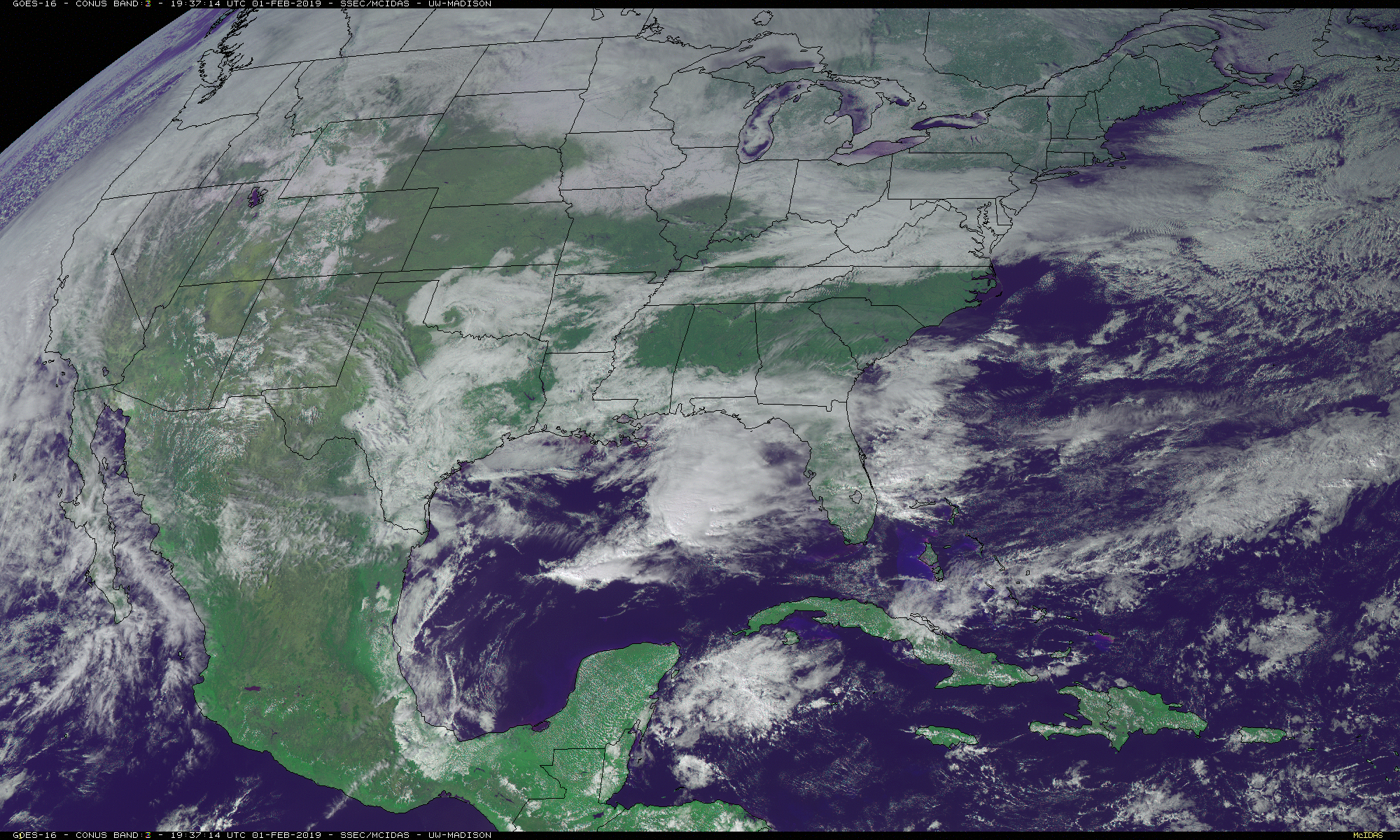
GOES-16 Full Color unadjusted for near-IR anomalous brightness--looks too green:
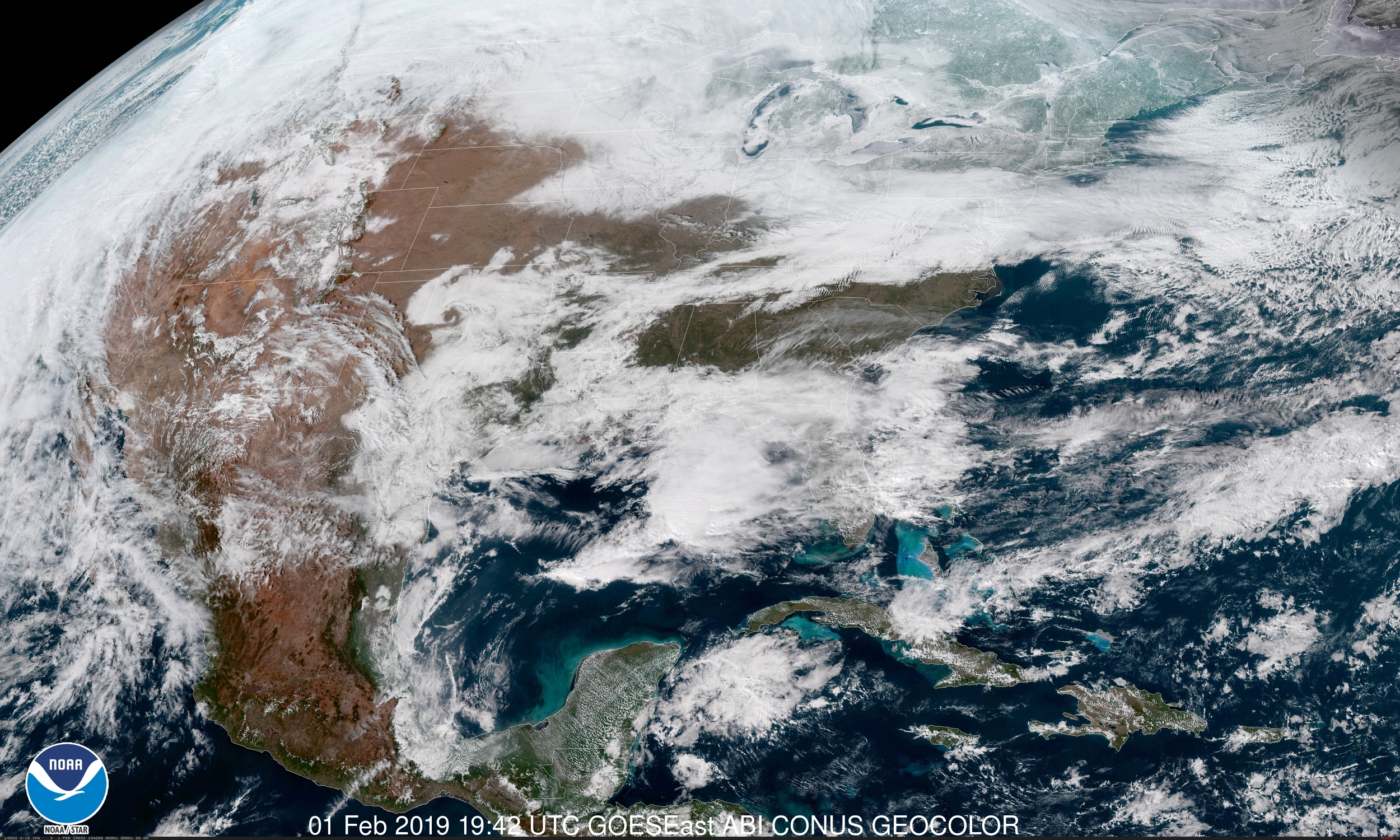
Appropriate adjustments can make the image more like what our eyes would see visually if we were sitting on the GOES-16 satellite; even though it is called "true" color on some websites, it is not true color because there is no actual green channel--choices must be made in how to substitute the near-IR channel for the green; the following image probably includes other adjustments as well:
A. Chosen in the spectral window region near 11 micrometers.
B. They are sensitive to IR radiation emitted from the earth's surface, or that emitted by clouds.
C. Radiation amounts measured by the satellite radiometer are stored as "brightness counts" in GVAR format (up through GOES-15). Brightness counts (iput) in GVAR format can be converted to radiometric temperatures using the inverse Planck function and a few corrections. They are presented as "equivalent blackbody temperatures," but commonly called "brightness temperatures."
D. In black and white satellite imagery
IR channels do not "see" fog very well, because fog is often close to the backround surface temperature.
- light shades correspond to cold, (usually) upper tropospheric brightness temperatures
- dark shades correspond to warm lower tropospheric brightness temperatures.
E. "Optically thick" clouds absorb radiation upwelling from the surface, blocking it from reaching the satellite. They emit IR radiation based on their cloud top temperature, and the satellite-observed brightness temperature is assumed to represent the actual temperature of the cloud top.
F. In clear areas, the brightness temperature is assumed to represent the temperature of the land or water surface.
G. "Optically thin" clouds such as cirrus may transmit some of the upwelling earth's surface radiation; the brightness temperature will represent a combination of both the cloud top temperature and the surface temperature, and come in somewhere in between.
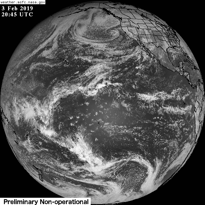
Example of a "heritage" GOES-15 IR image for the same time as the visible image above. There is a scale relating temperature in Kelvins to the gray shade. Note that nighttime areas that are black in the visible image show clearly evident cloud signatures in the IR.
Example of GOES-17 ABI Channel 13 10.3 micrometer "clean longwave window:"
Example of GOES-17 ABI Channel 14 11.2 micrometer "IR longwave window"--there is slightly more absorption by water vapor in this channel than in the "clean" IR window, but the images look nearly identical:
H. It should be noted that the conventional, historically common method of presenting IR images is essentially in negative. That is, the warmer, low-level scenes that emit more IR energy are shown as darker grey shades, while the colder scenes that emit less energy are presented as lighter grey shades (note the brightness temperature scale on the left side of the image):
If brightness of grey shades corresponded to brightness in terms of IR energy, the same image would look like this:
High, cold clouds are then dark (less energy) and low, warm land and ocean surfaces appear light (more energy).
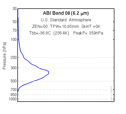
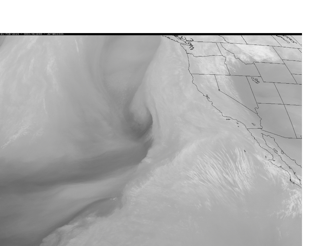
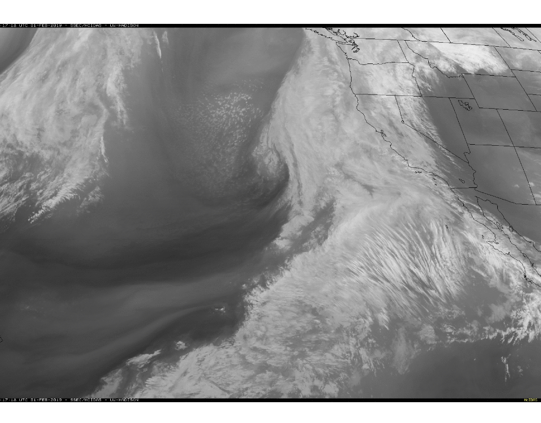
(3) Water vapor channels (heritage GOES-Imager Channel 3, 6.7 or 6.5 micrometers [see changes starting with GOES-12)], ABI Channel 8 6.2 micrometer "upper-level" water vapor, ABI Channel 9 "mid-level" water vapor, ABI Channel 10 "low-level" water vapor)
A. These channels are sensitive to IR radiation near 6.7 micrometers, the so-called water vapor absorption band of the thermal IR part of the spectrum.
B. In clear atmospheres, the upper-level channel senses radiation emitted from the upper 1-3 millimeters or so of column-integrated water vapor content of the air (also known as "precipitable water"). "Column-integrated" refers to the depth all the water vapor in each column of the atmosphere would have if it were condensed and its liquid depth measured. Typical values are 2-3 cm. Thus, the upper water vapor channel senses approximately the top 1-3 millimeters of it.
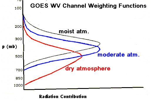
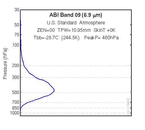
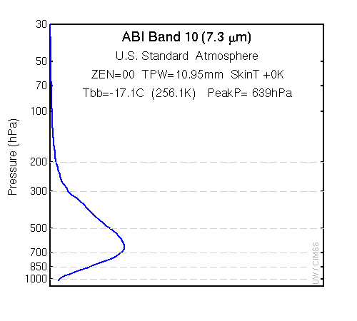
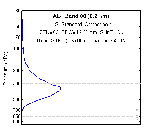
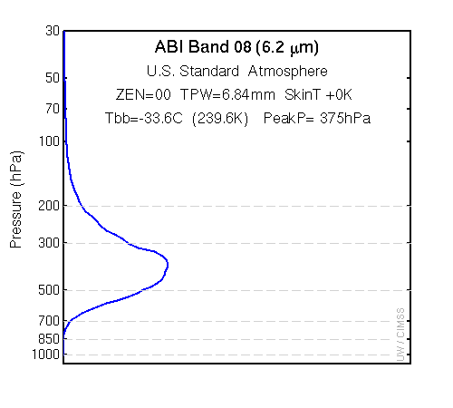
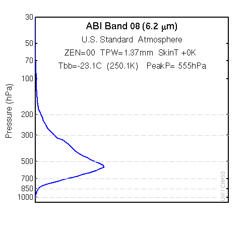
C. This condensed 1-3 millimeters is generally stretched out as vapor over roughly 500 mb of depth in the atmosphere, centered somewhere between the 400 and 500 mb levels, so the water vapor channels sense middle and upper tropospheric water vapor. The following figure shows an example of weighting functions for GOES-8 (former GOES-East) and GOES-12 (also former GOES-East) calculated from a "Standard Atmosphere." In general, weighting functions indicate how much layers at different altitudes in the atmosphere are contributing to the radiation measured by a particular satellite radiometer channel.
You can explore weighting functions of the GOES-16 water vapor channels using the following interactive page from the University of Wisconsin. Select Channel 8 as the channel that most closely emulates earlier GOES water vapor channels.
The upwelling radiation emitted by water vapor can be thought of as photons being emitted by individual water vapor molecules. Concentration of water vapor molecules decreases as height increases in the atmosphere. Generally photons from lower down in the atmosphere will hit another water vapor molecule and be absorbed before reaching the satellite. Photons emitted higher in the atmosphere are more likely to reach the satellite unimpeded because there are fewer molecules between them and the satellite. However there are also fewer molecules emitting radiation at high altitudes. Therefore, the peak of the weighting function occurs where there is the highest probability of a photon being emitted that has a clear, unimpeded path to the satellite.
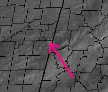
D. In tropical and midlatitude atmospheres, the upper-level water vapor channels typically do not "see" the earth's surface, or the water vapor below 600 or 700 mb except under very unusual conditions of extreme tropospheric dryness, as in this link for January 13, 2004 . Water vapor channel animations for January 13, 2004 showing the Great Lakes region and January 14, 2004 showing the northeast U.S. coastline reveal ghostly surface feature outlines due to extreme dryness attendant with extreme cold (surface temperatures of about -32C with dew point of about -35C at Pickle Lake, Ontario) that normally cannot be seen with the standard water vapor channel. The surface features here show up as temperature contrast between the warmer unfrozen water (darker) and the very cold land (lighter). Normally surface temperature differences would be completely obscured by intervening water vapor, but in this case there is so little water vapor in the air that we can see down to the surface features.
E. Water vapor channels also are sensitive to 6.7 micrometer radiation emitted by clouds. It is not always possible to distinguish clouds from water vapor in this kind of imagery.
F. In a typical greyshade enhancement, the following applies:
white/light shades--moist upper troposphere and/or high cloud tops--correspond to cold brightness temperatures/less radiation because radiation is coming from higher, colder regions (black curve on the contribution functions below)
black/dark shades--dry upper troposhere--correspond to warmer brightness temperatures/more radiation, because radiation is coming from lower, warmer regions (middle instead of high troposphere--red curve on the contribution functions below)
Chapter 2--Meteorological Satellites
A summary of the history of
the U.S. weather satellite programs is given here.
1. What do weather satellites do? Imaging,
sounding, and provide data for data assimilation.
Imaging is the process of
scanning successive positions over some portion of the earth's
surface with a radiometer taking individual radiation
measurements at each position, assigning a grey shade (or
colors) to each radiation value, then assembling the
measurements into a 2-dimensional image. Each pixel
represents one radiance measurement, in this case, expressed as
brightness temperature.
![]()
Satellite Sounding is the
process of deriving quantitative information about the vertical
distribution of atmospheric variables (such as temperature and
water vapor content), or "soundings," by remote sensing.
Conventional soundings are provided by radiosondes. This is
possible because different absorption channels obtain
information from different vertical layers of the atmosphere:
Satellite
soundings are not as accurate as radiosonde or aircraft
data, and suffer from lack of vertical resolution in comparison
with radiosondes. Sounding techniques were originally
developed for remote sensing of other planetary atmospheres such
as Venus, then adapted for meteorological purposes.
GOES Satellite sounding
Corresponding radiosonde sounding.
Data assimilation is the process of
quantitatively incorporating satellite-measured radiance
information into numerical weather prediction model
initial-analysis fields to improve the spatial
distributions of temperature and water vapor in data-sparse
regions. Whereas direct incorporation of satellite-derived
soundings into the models often actually degraded(!)
model forecast performance, direct assimilation of the radiances
has been shown to improve the model forecasts, especially in
regions with sparse radiosonde coverage like the oceans.
Data assimilation uses the model initial atmosphere (usually
derived from a combination of radiosonde and aircraft
observations and a previous model forecast for that time) as
input to radiative transfer models to calculate radiances that
particular satellite channels should measure if viewing that
atmosphere. Where there are discrepancies between the
model-calculated radiances and the satellite-measured radiances,
model vertical distributions of temperature and water vapor are
adjusted to bring calculated radiances into alignment with the
satellite radiance.
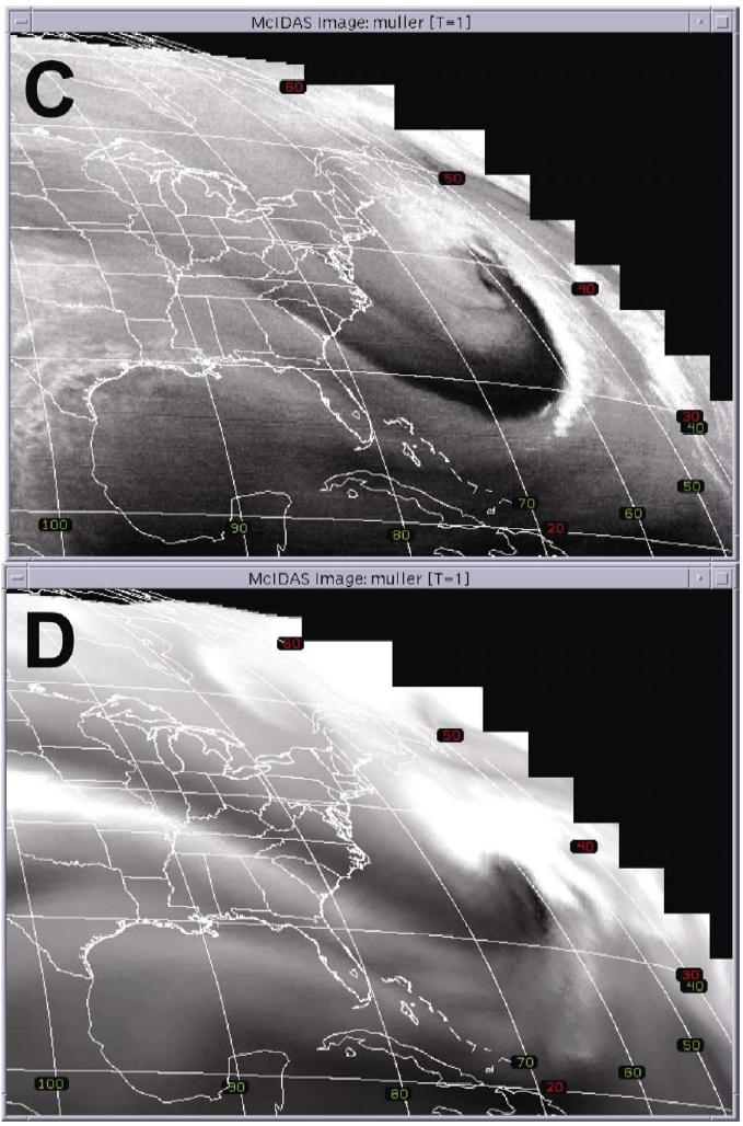
Observed vs. calculated radiance images--the model initial water
vapor and temperature fields might be adjusted for the
discrepancy in the location of the dark streak (dry upper air)
being farther south in the real image than in the simulated
image:
To summarize:
2. There are two main types of weather satellite orbits, polar (sun-synchronous) and geostationary (geosynchronous):
A. Polar orbit. Passes close to poles. Altitude of roughly 800 km.
(1) Orbit is "sun-synchronous". It stays in same orientation with respect to the sun while the earth rotates underneath.
Image credit: NASA Earth Observatory
(2) Ascending node is the south-to-north pass over the earth's surface. Descending node is the north-to-south pass.
(3) Recent U.S. series of polar orbiting weather satellites are the NOAA series of satellites primarily for civilian weather applications, and the DMSP (Defense Meteorological Satellite Program) primarily for military use, although data from both have been shared between the civilian and military sectors. They contain visible, conventional IR, and IR water vapor channels, as well as microwave channels. They have provided the backbone of satellite capabilities for sounding and data assimilation into numerical weather prediction models, and also provide images that are especially useful in polar regions that geostationary satellites only cover poorly or not at all.
(4) The polar orbiting weather satellites take around an hour and 40 minutes to circle the earth; for example, NOAA-19, launched in 2009, has an orbital period of 102.14 minutes.
(4) A new generation of polar orbiting weather satelllites has been initiated with the launch of the Suomi NPP (the National Polar-orbiting Partnership, formerly the NPOESS [National Polar Orbiting Environmental Satellite System] Preparatory Project) satellite launched October 28, 2011 (see also the Suomi NPP entry in Wikipedia). It was intended as a developmental satellite to transition from the NOAA and DMSP series of satellites to the JPSS (Joint Polar Satellite System) program, meant to reduce duplication between the military and civilian satellite programs. Ultimately, however, the Department of Defense participation was dissolved, and the JPSS was launched November 18, 2017. and is now known as NOAA-20, the first of a new generation of operational polar orbiting weather satellites.
B. Geostationary orbit. Stays over a single spot on the equator. Altitude of roughly 36000 km (22000 mi).
(1) Orbit is "geosynchronous". It orbits directly over the equator at such a rate that it stays over the same spot on the earth all the time.
The point on the earth directly underneath is called the satellite subpoint.
Satellites in geostationary orbit must be directly over the equator.
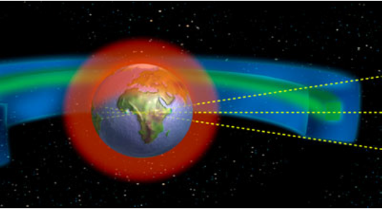
The Interagency Space Debris Coordination Committee (IADC) defines the "geosynchronous region" as
"A segment of the spherical shell defined by the following:
Lower altitude = geostationary altitude minus 200 km
Upper altitude = geostationary altitude plus 200 km
-15 degrees ≤ latitude ≤ +15 degrees
where geostationary altitude is defined as 35,786 km"
Within the geosynchronous region is the "geostationary belt, defined as a circular orbit 35,786 kilometers in altitude above the Earth with an inclination of zero (meaning it is directly over the Equator)."
--from https://goes.gsfc.nasa.gov/text/Zombiesats.pdf
The blue area above is the "geosynchronous region", while the green is the "geostationary belt." The geostationary belt is limited and thus is very valuable for space operations for communication satellites, weather satellites etc. It is therefore managed by the International Telecommunications Union who coordinates assignment of radio frequencies and satellite slots in geostationary orbit. "Slots" are 2 degrees of longitude or about 1470 km. Satellite operators maintain a satellite within its slot within an "orbital box," typically around 0.1 deg of longitude or 70 kilometers in length.
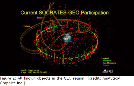
When a geostationary satellite is no longer operational it is supposed to be "disposed of" by moving it out of geostationary orbit by forcing it into an inclined orbit to avoid collisions and radio frequency interference with the active satellites. In the figure below only the green and orange dots represent active satellites. The rest is debris. As of 2010, out of approximately 1200 known objects, there were roughly two debris objects for every active satellite! Note that as of the below figure, we could only detect objects larger than a basketball.
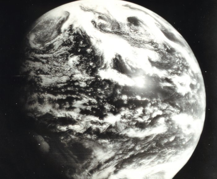
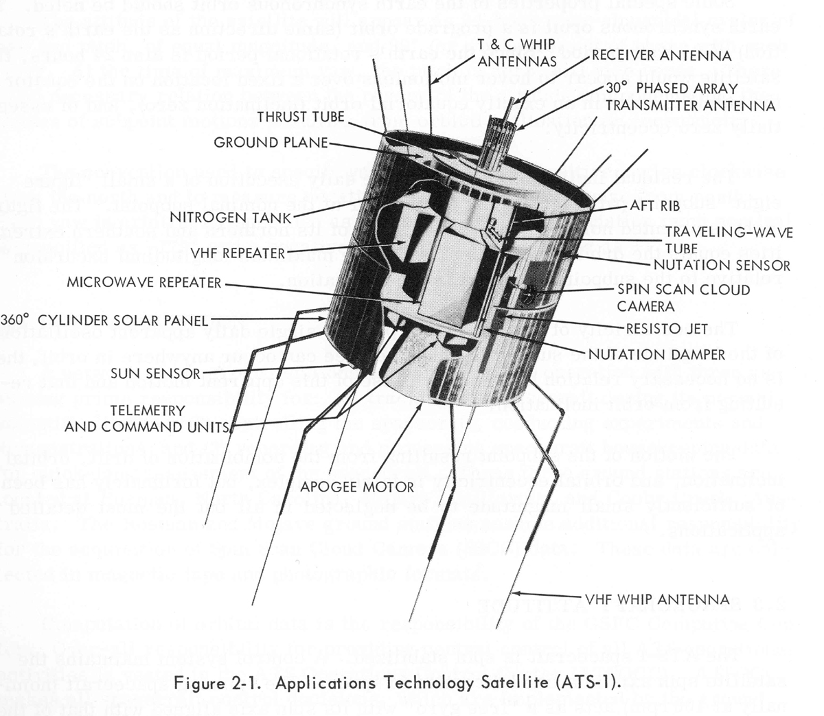
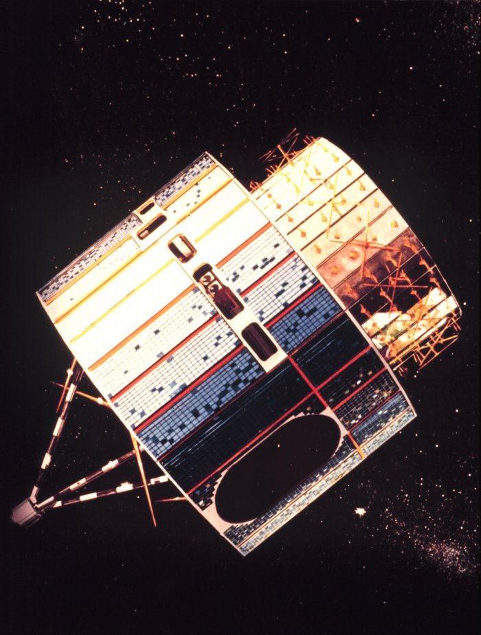
(2) The first geostationary satellite to carry a weather instrument was the ATS (Applications Technology Satellite series carrying the Spin-scan cloudcover camera, first launched in December, 1966. These were prototypes to demonstrate geostationary capabilities for a variety of applications, not just weather.
This was followed by the SMS (Synchronous Meteorological Satellite) series, the first geostationary satellites devoted to meteorological observations, and first launched in May, 1974.
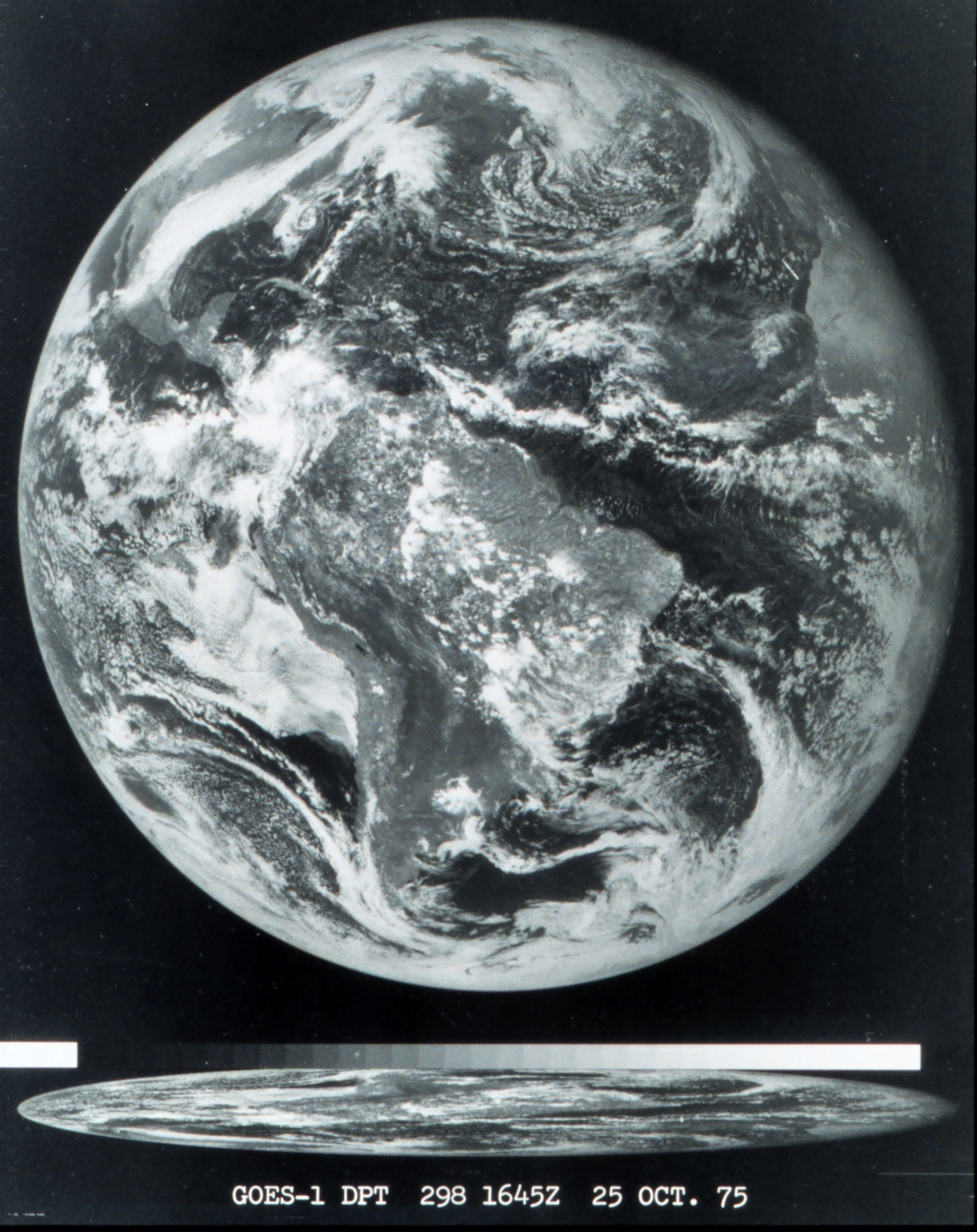
These were prototypes for the original series of GOES(Geostationary Operational Environmental Satellites) satellites, GOES 1-7, first launched on October 16, 1975. GOES 1-3 were essentially identical to the SMS. Like the ATS and the SMS they were "spin-scan" satellites, and contained the Visible Infrared Spin-Scan Radiometer (VISSR).
GOES 4-7 contained a new instrument, the VISSR Atmospheric Sounder (VAS), allowing for the measurement of vertical profiles of temperature and water vapor.
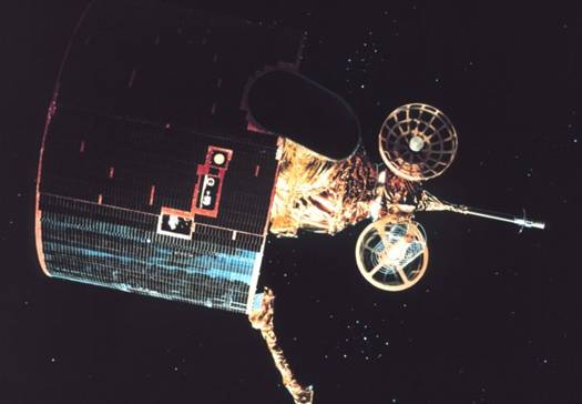
The satellites are normally designated with a letter prior to launch, which is changed to a number after launch. Upon launch, the GOES I-M series became GOES 8-12, while the GOES N-P series became GOES 13-15). These series are very different than the previous generations in that they are 3-axis stabilized satellites, not spin-scan like the previous series.
They contain visible, IR, and water vapor channels for both imaging and sounding. In this class we are mainly concerned with imaging, including the channels on the "legacy" GOES Imager instrument, and most importantly, their analogs on the current ABI (Advanced Baseline Imager) instrument. The table in the following link (GOES Imager characteristics and uses) GOES imaging channels 1-5 (and 6 replacing 5 , their spectral bands, and what they are used for.
(3) Currently, GOES-16 is the "GOES-East" component of the U.S. geostationary satellite system, centered over the Atlantic Ocean at 75o west, with the previous GOES-East, GOES-13, serving as backup. GOES-15 is the "GOES-West" centered over the Pacific at 135o west .
GOES-13 was launched on May 24, 2006 and reached geostationary orbit containing 15 years of geosynchronous station-keeping fuel. It was placed into on-orbit storage in January 2007 ready to replace the GOES-12 or GOES-11 as needed. In December 2008, GOES-13 briefly was activated when GOES 12 suffered a communication outage due to a thruster malfunction. GOES-12 resumed Operational East Status on 1/06/2009 at 15:00z, and GOES-13 was returned to on-orbit storage. On May 14, 2010, GOES-13 replaced GOES-12 as GOES-East, since it was feared that GOES-12 would not remain reliable through the 2010 hurricane season. GOES-12 then was moved westward to routinely scan South America and the full earth disk. On August 16, 2013, after a 10 year operational lifetime (5 years longer than planned!), GOES-12 was decomissioned. GOES-14 (formerly GOES-O) was launched June 27, 2009, has undergone post-launch check-out, and is currently on standby. It was briefly brought out of storage during Fall, 2012, while GOES-13 was malfunctioning, and was being moved into position to become the new GOES-East satellite, but then GOES-13 was fixed, and GOES-14 was put back into storage at 89.5o west. GOES-15 (formerly GOES-P) is the current GOES-West satellite. It was launched March 4, 2010, and subsequently completed 5 months of post-launch testing. It was placed on standby along with GOES-14, but was moved into place at 135 degrees west longitude, replacing GOES-11 as the operational GOES-West satellite on December 6, 2011. On December 18, 2017, GOES-16 replaced GOES-13 as the operational GOES-East satellite. Information on all the current GOES satellites and their status can be found at the NOAA Office of Satellite and Product Operations GOES Page.
Click below for global visible and IR views from both GOES-East and -West:
GOES-East VIS
GOES-East IR
GOES_West VIS
GOES-West IR
The launch history and current status of the GOES I-M and N-P series spacecraft:The first of the new GOES R-U series was launched as GOES-16, Nov. 19, 2016:
- GOES-8 (I) - launched 13 Apr 1994 - decommissioned (Apr 2003)
- GOES-9 (J) - launched 23 May 1995 - decommissioned (Jun 2007) (at 160E)
- GOES-10 (K) - launched 25 Apr 1997 - decommissioned (Dec. 2009) (at 60W)
- GOES-11 (L) - launched 03 May 2000 - decommissioned (Dec. 16 2011) (4.5 deg/day westward drift)
- GOES-12 (M) - launched 23 Jul 2001 - decommissioned (Aug. 16 2013)
- GOES-13 (N) - launched 24 May 2006 - became backup GOES-East on Dec. 18, 2017 (at 75W) Originally scheduled for launch in 2001: Read the incredible saga of the GOES-13 launch here.
- GOES-14 (O) - launched 27 June, 2009 - standby (at 105W, after briefly becoming operational for GOES-13 during Fall, 2012 and briefly again after GOES-13 suffered a meteor collision on 22 May 2013))
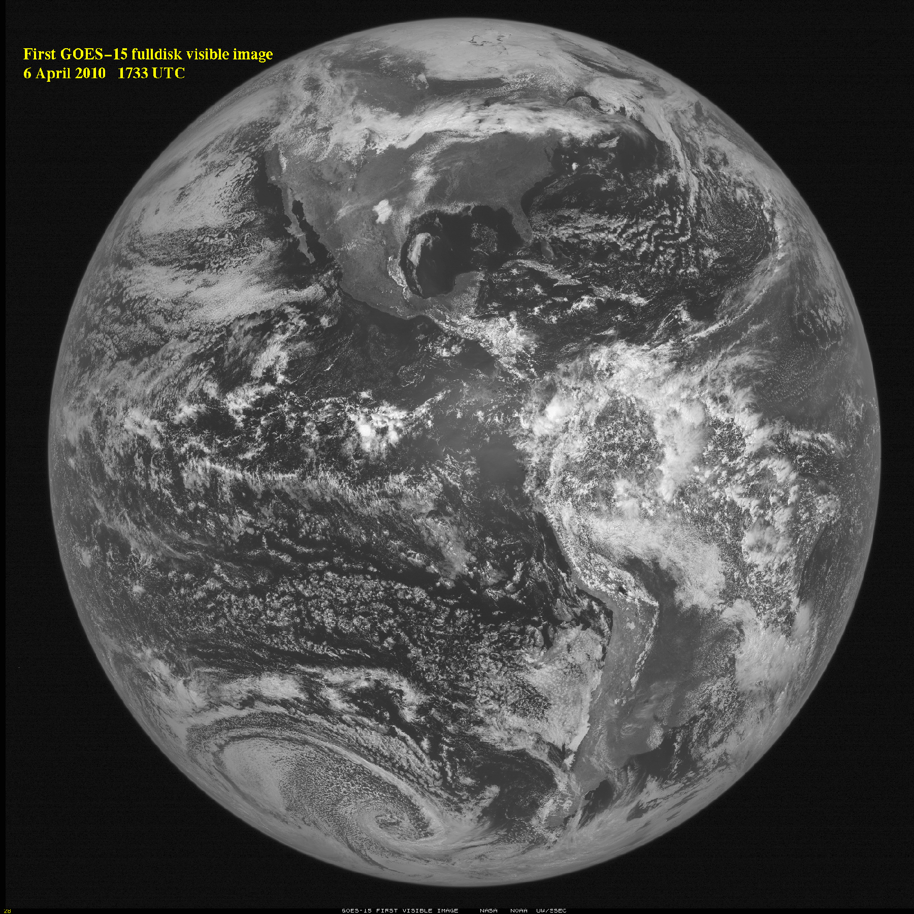
- GOES-15 (P) - launched 4 March 2010 - operational GOES-West (at 135W) starting on Dec 6 2011.
GOES R-U is a new generation of geostationary satellites and has many new and improved capabilities compared with the GOES I-P series, including:
- GOES-16 (R) - launched November 19, 2016 - is now operational GOES-EAST starting on December 18, 2017 at a longitude of 75.2W. It contains the Advanced Baseline Imager (ABI), a 16 channel imaging radiometer compared with the old GOES Imager, a 5 channel radiometer.
- higher resolution
- the Advanced Baseline Imager (ABI--16 channels vs. 5 on the "heritage" GOES imagers)
- more frequent data
- a Geostationary Lightning Mapper (GLM)
- a "space weather" suite of instruments
- GOES-17 was launched on March 1, 2018 and originally scheduled to replace GOES-15 as the operational GOES-West weather satellite during Fall 2018. However, a radiometer cooling system issue was discovered impacting some of the IR channels, and delaying the transition to operations. In November, 2018, GOES-17 was moved to its operational position at 137.2W. The government shutdown further delayed the transition to operations, but the satellite finally became the operational GOES-West on February 12, 2019.
The view from the GOES satellite configuration as of September 2018 during testing of the GOES-17 when it was located near the position of GOES-16, is as follows:
From left to right, GOES-17, GOES-16, and GOES-15, respectively:
GOES-17 after its move to its operational position at 137.2W longitude during October and November 2018, but before it became operational GOES-West during on February 12, 2019:
(4) The early spin-scan versions of GOES up through GOES-7 scanned the earth by sweeping across on each scan, taking about 1/2 hour to scan the entire earth disk. This meant that the satellite was pointing at the 18 degree disk of the earth (the angular width of earth from geostationary altitude) for only 5% of its operational time during one 360 degree rotation. The three-axis stabilized versions of GOES starting with the GOES I-P series were intended to improve the scanning budget by pointing at the earth continuously. The GOES I-P series created images of the earth by scanning east-to-west then stepping down (south) and scanning west-to-east etc. (image borrowed from the no-longer-available GOES pages of Daphne Zaras):
Each individual field-of-view overlaps the previous measurement on the scan by half, but the scan line does not overlap the previous scan line in the north-south direction. Unfortunately it took these versions of GOES 26 minutes to scan the entire earth disk, not really an improvement over the spin-scan versions of GOES. This problem was solved by rearranging the scanning budget to scan limited sectors more frequently, yielding routine CONUS imagery every 15 minutes.
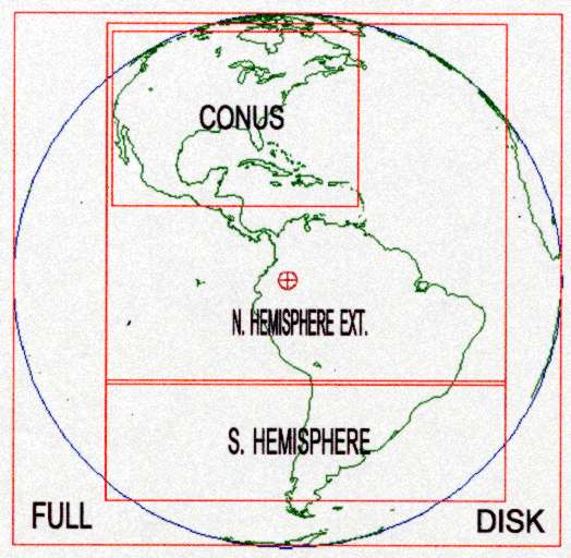
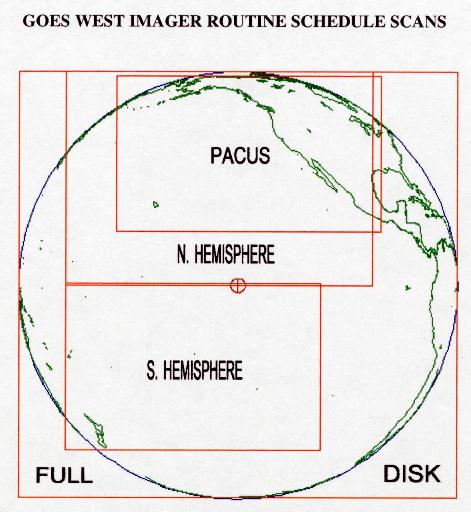
(5) Up through GOES-13, GOES-East routinely scanned the following earth sectors on this previous GOES-E schedule:
Scanning the full earth disk took 26 minutes, while scanning the continental United States (CONUS) took nearly 5 minutes. Routine scanning yielded CONUS images every 15 minutes, and full disk images every 3 hours.
Details on scanning strategies are found on NOAA Office of Satellite and Product Operations of NESDIS (National Environmental Satellite Data Information Service).
Two additional scanning strategies are RSO (Rapid Scan Operations [click on Rapid Scan Overview and Rapid Scan Operations] ) and SRSO (Super Rapid Scan Operations [click on Super Rapid Scan Overview and Super Rapid Scan Operations] ). A description is provided by the NASA Goddard Space Flight Center:
     In the GOES routine schedule scan mode, two views at approximately 15
     minute intervals of the CONUS (GOES-8 [now replaced by GOES-12]) or
     PACUS (GOES-9 [now replaced by GOES-10]) are provided in a
     half hour period.  A northern hemisphere scan is also included in the 30
     minute cycle.

     During GOES Rapid Scan Operations (RSO), 4 views of the CONUS (GOES-8) or
     Sub-CONUS (GOES-9) are provided at approximately 7.5 minute intervals in a
     half hour period.  A northern hemisphere scan for both GOES is also
     included in the 30 minute cycle.

     During GOES Super Rapid Scan Operations (SRSO), approximately 10 one minute
     interval scans are provided every half hour using prescribed 1000x1000km
     sectors.  The remaining time in the half hour cycle is devoted to scans of
     the northern hemisphere and CONUS (GOES-8) or Sub-CONUS (GOES-9).

     When GOES RSO or SRSO is utilized, most of the southern hemisphere is not
     scanned.
The rapid-scan strategies are used for severe weather monitoring.
Similarly, GOES-West routinely scanned on the following sectors on this schedule:
These links give GOES-West RSO (Rapid Scan Operations [click on Rapid Scan Overview and Rapid Scan Operations] ) and SRSO (Super Rapid Scan Operations [click on Super Rapid Scan Overview and Super Rapid Scan Operations] ) information.
**The GOES-16 ABI instrument, now operational GOES-East can cover the earth much more rapidly because it has more detectors working simultaneously (8000 detectors on the GOES-ABI vs. 16 on the GOES-I-P Imager). Currently, GOES-16 operates in Routine Scan Mode 6, also known as Flex Mode, delivering a full disk scan every 10 minutes, CONUS images every 5 minutes, and two floating mesoscale sectors, each with images every 1 minute that focus in on operationally significant events like Hurricane Florence, for example. The meso sectors are offset from each other by 30 seconds, so both mesoscale sectors Meso1 and Meso2 can be pointed at the same location to provide imagery every 30 seconds. Routine Scan Mode 4, also known as Full Disk Mode yields full disk imagery every 5 minutes.**
ABI Flex Mode Full Disk sector--every 10 minutes.
ABI Flex Mode Conus Sector--every 5 minutes.
ABI Flex Mode Meso1--every 1 minute.
(6) Other countries' geostationary satellites have included the following (data from many of them are available on the internet):Himawari series: successor to the MTSAT series, which was the successor to the GMS--Japan. Western Pacific ocean. Useful for typhoons, Asian weather. The Himawari imaging radiometer is called the AHI (Advanced Himawari Imager) and is similar to the GOES-ABI, but has a green channel at 0.51 micrometers for true color.
INSAT--India.
MSG (METEOSAT Second Generation), successor to METEOSAT--European Space Agency. Coverage of Europe, Africa, and the eastern Atlantic Ocean.
GOMS--Russia.Combining imagery from some of these satellites can produce a global mosaic with coverage as follows:
Feng-Yun-2 (FY-2)--China
COMS or KOMPSAT--Korea
Simulations of the current view of earth (not actual satellite images!) from these satellites can be viewed via this website.
1. Image composition.
A. Wx satellite images are composed of thousands of pixels (short for "picture elements")--tiny rectangles, each composed of a single shade of grey (representing a single brightness value [expressed as "brightness counts"] or amount of measured radiation).
As an example, the following is an enhanced grey-shade IR image of Hurricane Rita; the scale on the left shows the association between the brightness counts and the "brightness temperature" in degrees celsius:
Zooming in we can begin to see the pixelated structure of the image:
(1) A single pixel represents the average brightness value over the area covered by the pixel.
(2) Contrast is the degree of grey tone difference between two pixels. Greater contrast makes features easier to distinguish.
(3) Resolution refers to the size of the smallest feature that can be seen in an image. Since one pixel is the smallest element in an image, the distance represented by the dimensions of a pixel is the image resolution.
(4) The reported or nominal resolution of an image refers to that at the satellite subpoint (i.e., the point on earth directly beneath the satellite). The above images of Hurricane Rita have a nominal resolution of 4 km. However, the actual resolution decreases as you move away from the satellite subpoint due to the change in viewing angle. Therefore each pixel in the above images has dimensions greater than 4 km.
(5) Terminology can be confusing: high resolution refers to small features being resolved, while low resolution refers to the ability to resolve only large features.
An unenhanced image has a simple,
single-slope, straightline mapping of
image radiances (expressed as brightness counts or brightness
temperatures representing individual radiation
measurements) to grey shades as shown in the following
curve:
On this curve "counts (input)" refers to the
raw radiation amounts measured by the satellite at
individual pixels, while "counts (output)" refers to the
grey shade for display assigned to the input counts.
For example 150 input counts is displayed as 150 output
counts on an unenhanced image.
In a nutshell:
counts (input) is what is measured
(representing radiance
values)
counts (output) is how it's displayed
[Note: The satellite stores measured
radiation as digital values in a binary
format as a sequence of 1's or 0's. A previous
generation of GOES satellites used 8-bit "words" meaning
that an 8 place sequence of 1's or 0's represents a maximum
of 256 ( 28 ) different values from 0 to 255,
hence the ranges seen in the figure above. The more recent
generation of GOES satellites up through GOES-15 used 10-bit words, meaning
that 1024 ( 210 )
different values can be represented; the GOES-ABI has capacity for 214 = 16384 different values, but depending on the channel downloads anywhere from 211 to 214 of those values and discards the bits that are within the noise of the measurement]
Enhancement refers to the remapping of image brightness
values to grey or color shades and is explained in the Image
Enhancement
Tutorial . You should be familiar with the
concepts of enhancement as described in class using the
tutorial and understand how simple changes in an enhancement
curve will affect the appearance of a satellite image.
The figure below gives an example of
using the enhancement curve to remap brightness values:
The ZA enhancement is shown in black while
the green lines show the original unenhanced curve; note
that from roughly 100 to 200 input brightness counts, the ZA
curve is identical to the unenhanced version.
Following the blue path up from 60 input counts or down from
25oC we see that the unenhanced curve yields 60
output counts (remember, input counts or brightness
temperature correspond to measured amount of radiation while
output counts correspond to how it is displayed in grey
shades). On the ZA enhancement we see that 60 counts input or brightness temperature 25oC now
corresponds to 30 counts output, a darker shade.
Actual grey shades corresponding to 60 vs. 30 output counts,
respectively are shown here-- 60:  30:
30:

More importantly, notice that the entire input range of
50-100 counts has now been "stretched" over an output range
of 0-100 counts, increasing the displayed contrast of this
input range:


A physical interpretation of the ZA enhancement is that it accentuates contrast for the temperature range of the surface and lower troposphere (the steepened lower part of the curve), does not affect how midtropospheric temperature ranges are displayed (unchanged middle part of the curve), and accentuates contrast for the temperature range of the upper troposphere/tropopause (upper part of the curve).
Click on this link to see a list of image
enhancement curves and what they are used for: Enhancement
Curves
List.
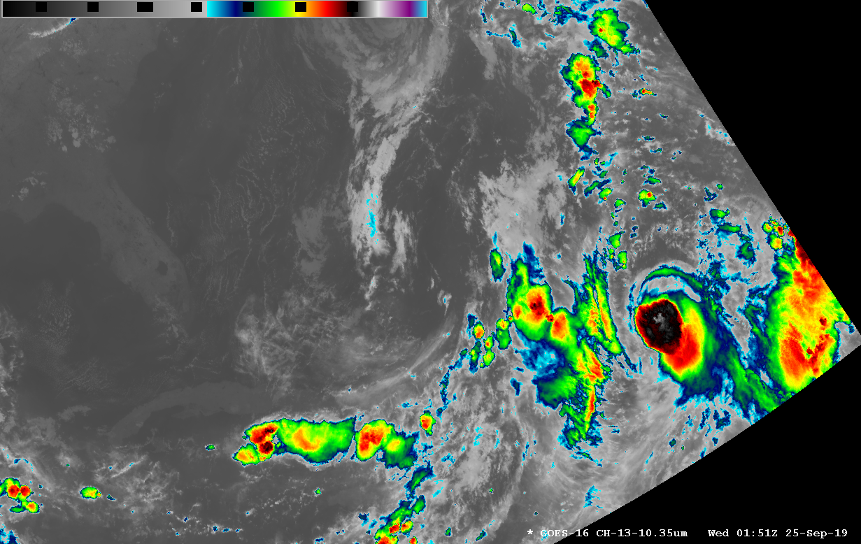
Currently-used image enhancements are mostly color-enhancements. Most IR enhancements for longwave IR window channels are designed to highlight high, cold cloud tops and convection:
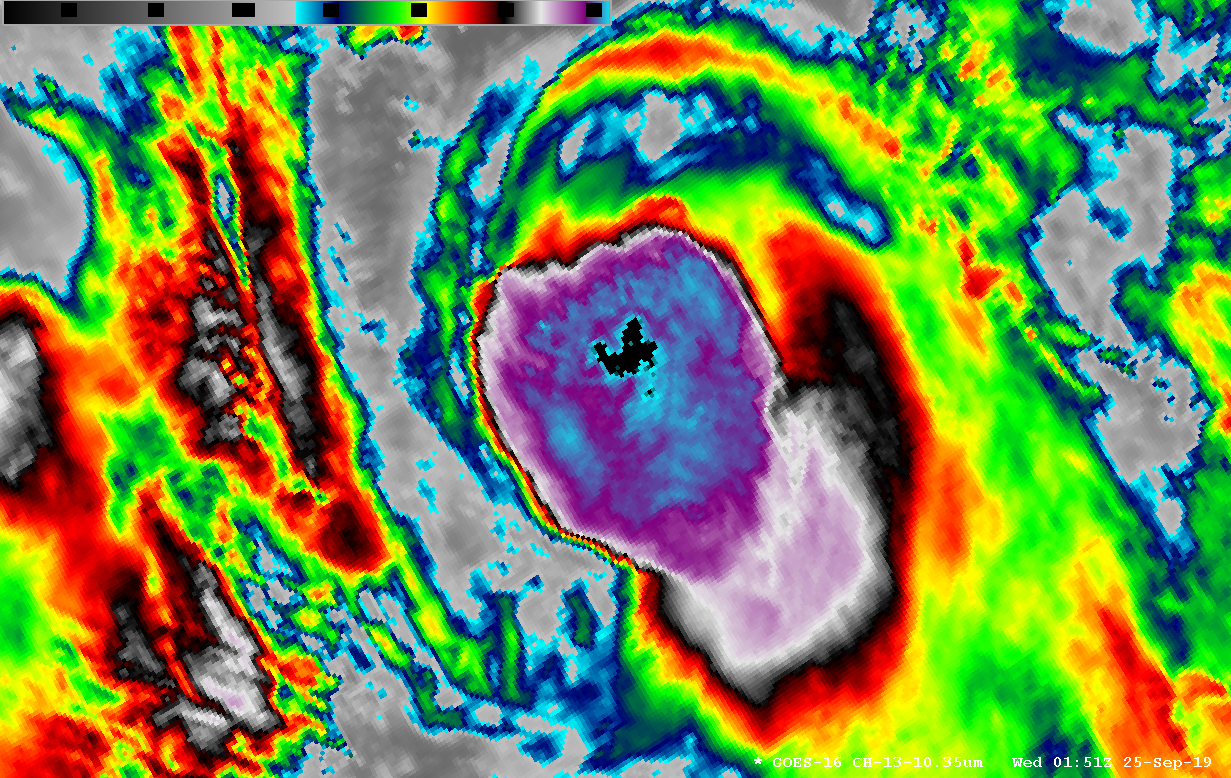
AWIPS can be used to adjust enhancements and make features such as overshooting thunderstorm tops stand out:
The following is an example of an image enhancement scale that was designed to convey visual information from all three different ABI water vapor channels using the same scale:
Ch. 8 upper level water vapor: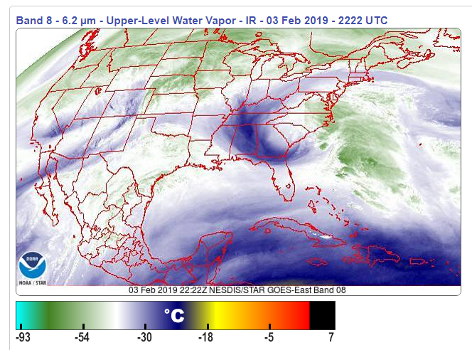
Ch. 9 middle level water vapor: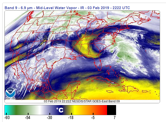
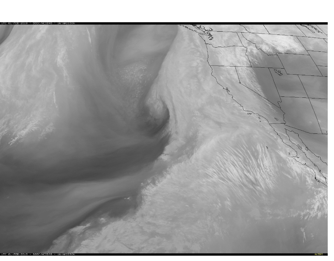
Ch. 10 lower level water vapor: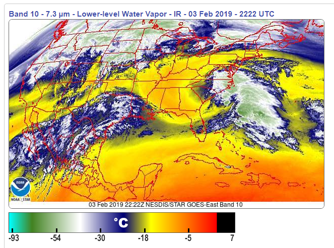
Errors in Satellite Imagery
Can be caused by sensor limitations, viewing angle, and parallax shifting.
Cloud displacement.
Unless a cloud is at the satellite subpoint, the viewing angle of the satellite will cause the apparent location of the cloud to be displaced from its actual location:
Note the displacement between the following radar and satellite images of and overshooting thunderstorm top in satellite imagery vs. the location of the reflectivity maximum in the radar. Due to the satellite view from the equator, the overshooting top appears farther north than the reflectivity maximum:
This loop shows the effect of parallax on displacement of image features. It was (created by Dr. Fred Mosher using McIDAS).
An approximate rule of thumb is that the displacement error of a feature in midlatitudes is about equal to its height.
Limb Darkening
"Limb darkening" refers to a decrease in measured amounts of radiation by a satellite radiometer as the viewing angle increases away from the satellite subpoint. It is most pronounced on the edges or "limbs" of the satellite image.
Out on the "limbs" of the image, the path between a scene being viewed and the satellite radiometer traverses more of the atmosphere; more radiation is absorbed by the
intervening atmosphere or is scattered out of the path and does not make it to the radiometer. This makes the scene appear colder than it actually is (less radiation reaching the radiometer).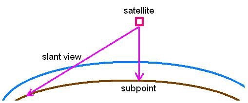
Note: The term limb "darkening" refers to lower radiation amounts/cooler brightness temperatures. However, because we DISPLAY such cooler TB's as lighter grey shades or brighter colors, limb "darkened" portions of images acually LOOK brighter than they otherwise would!!